

Tutorials on electrochemical measurements #1- Parameter selection for electrochemical impedance spectroscopy
- Jul 6, 2025
- 10 min read
Updated: Jul 7, 2025
Here is Edward Bear, coming downstairs now, bump, bump, bump on the back of his head, behind Christopher Robin. It is, as far as he knows, the only way of coming downstairs, but sometimes he feels there really is another way, if only he could stop bumping for a moment and think of it.
A. A. Milne. Winnie the Pooh.
Aim of the tutorials
Electrochemical sensors have different challenges compared to other sensing methodologies. Consider optical measurements, where your sample never directly contacts the photodiode, and system issues remain largely independent of the chemistry involved. Whether red light originates from photons interacting with a tomato or haemoglobin makes no difference to your optical components. But in electrochemistry the key focus is on the interaction between the sample and electrodes. The measurement system itself becomes part of the chemistry.
In the most basic terms, in electrochemical systems changes in electric fields induce chemical changes, and conversely, chemical interactions generate electrical signals through process like electron transfer between molecules and metals. This principle forms the foundation of electrochemical sensors. See Figure 1 for working principle of affinity-based sensors, though other techniques exist as well.
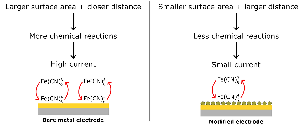
Considering figure 1, when you introduce a redox couple such as potassium ferro/ferricyanide to a bare metal electrode, complex interactions occur involving mass transfer, diffusion, and electron transfer (for more details, see references). These interactions are localised, occurring at dimensions as small as 10 nanometers for example. This nanoscale sensitivity is a powerful sensing opportunity. Even tiny molecules covering the electrode surface can significantly impede the redox couple's access to the electrode, reducing interactions and consequently decreasing the generated current. This principle underlies many biosensor designs, where target molecules and biomarkers, which typically only a few nanometers in size, are too small for conventional impedance analysers to detect directly. However, the molecular blockage of electrode surface provides sufficient interference with electron transfer to generate measurable signals. By making correlations between current and concentration, we can quantitatively determine target molecule concentrations, making electrochemistry both convenient and powerful for sensing applications.
But things are not that easy. Despite these advantages, electrochemical systems are far from straightforward. They exhibit non-linear behavior and other complicated stuffs such as biofouling, washing steps, and sensitivity to temperature and pH. Developing a reliable electrochemical sensor is often like making Rube Goldberg's "self-operating napkin". The cartoon depicts an elaborate chain reaction designed to automate a simple task, but it rarely functions in reality. For example, the bird never sits there. This analogy is also suitable for electrochemical sensors. Achieving repeatable, stable, and sensitive measurement requires the precise coordination of multiple disciplines: from electronics and software to chemistry and biology. This multidisciplinary complexity makes sensor development particularly challenging.

Here our aim is to share the lore of electrochemical measurements from the point-of-view of a biosensor start-up for engineers, scientists, and enthusiasts with a shared passion for sensor development. At the upcoming tutorials we will delve into more details of important topics starting from basic calculations to signal processing for sensor development and bringing up an electrochemical system. Theory, design and experiments will be included in the tutorials.
Introduction
This tutorial focuses on the fundamentals of electrical parameter selection for electrochemical impedance spectroscopy (EIS). While sensor development has far more complexity than parameter selection alone, understanding these basics provides essential groundwork for successful EIS implementation. Future tutorials will explore both theory and experiments of electrochemical measurements in greater depth.
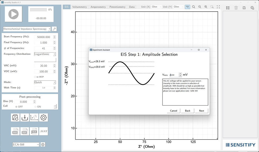
With that big picture in mind, let’s dive straight into the tutorial. Let's start by opening "Experiment Assistant" from Sensitify Studio. Click the button shown with the arrow in Fig. 3.

After selecting "Electrochemical impedance spectroscopy" from the drop-down menu, click "Next":

Step #1: Amplitude selection
Impedance is defined as the ratio of voltage to current: Z = V/I. In electrochemical impedance spectroscopy, we apply a voltage signal at a specific frequency to the sensor and measure the corresponding current response. Dividing the applied voltage by the measured current yields the impedance at that frequency. From a signal-to-noise ratio perspective, applying larger voltages would seem advantageous since higher voltages generate larger currents, making measurements easier and improving the signal-to-noise ratio. However, this approach has a fundamental limitation in electrochemical systems.
Electrochemical sensors are inherently non-linear systems. A system is considered linear if it satisfies this condition: f(ax + by) = af(x) + bf(y). In practical terms, if we apply a 1 kHz input signal to a linear sensor, the output will also be a 1 kHz signal. Non-linear systems, however, produce outputs that deviate from this relationship.
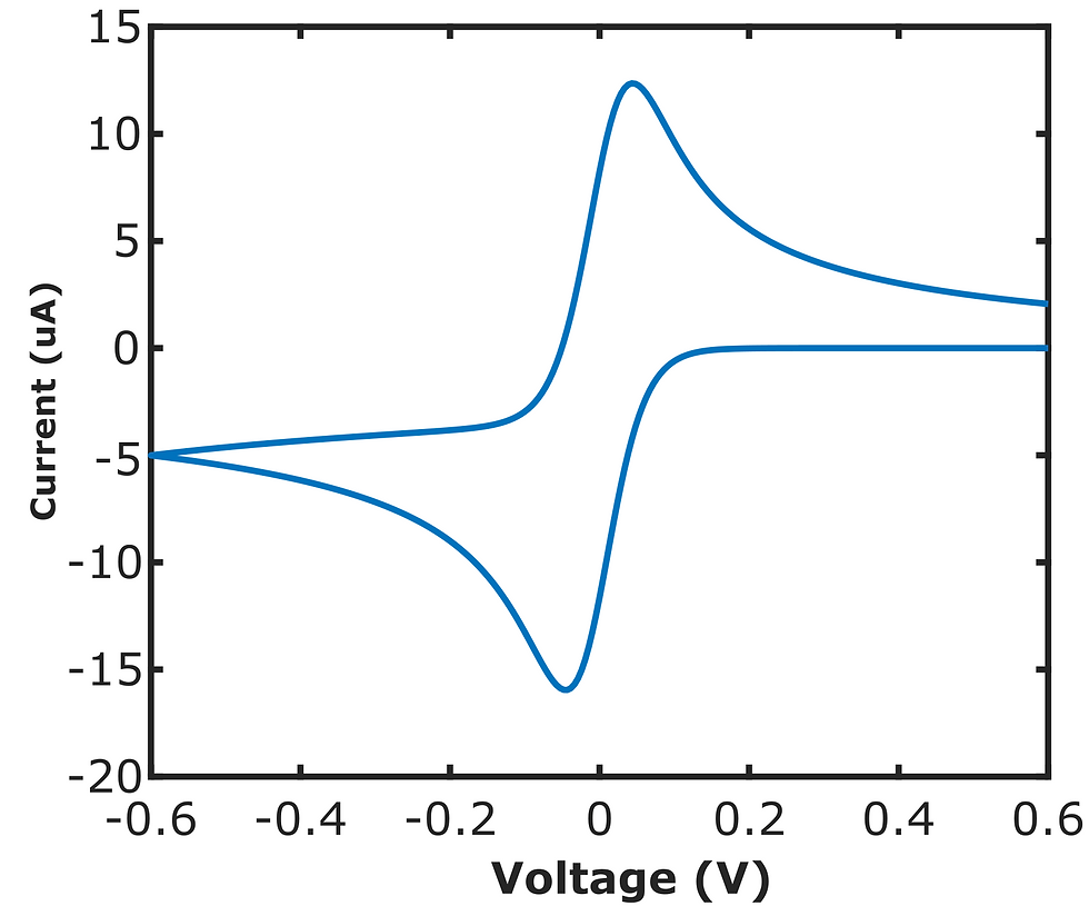
Cyclic voltammetry (CV) provides a clear illustration of this non-linearity. In CV experiments, a single voltage value often corresponds to two different current values—one during the anodic sweep and another during the cathodic sweep (see simulation figure below). For instance, at 0.15 V, we might observe an anodic current of 13 μA and a cathodic current of -17 μA. This raises a fundamental question: which current value should we use to calculate impedance? Is it 0.15V/13μA or 0.15V/-17μA? This ambiguity demonstrates why traditional impedance calculations fail for non-linear systems. While methods exist for analyzing non-linear systems, the vast majority of researchers and engineers rely on linear analysis due to the abundance of well-established engineering and mathematical tools, such as Fourier transform, available for linear systems.
Fortunately, we can still calculate impedance for non-linear electrochemical systems using small-signal analysis. This approach involves applying a very small signal to the sensor to obtain correspondingly small changes in response. Within this limited range, even non-linear sensors behave approximately linearly, enabling accurate impedance calculations. The primary criterion for selecting AC amplitude is therefore satisfying the linearity condition. However, this isn't the only consideration: the applied voltage can also trigger molecular interactions at the electrode surface, potentially leading to unexpected results (remember our Rube Goldberg machine analogy)

Okay, so we should choose an amplitude value which is high enough for satisfying linearity condition. How can we check this condition? There are different methods for this purpose, and these 3 are the most populars:
Using Kramers-Kronig relations
Testing at different amplitudes
Circuit-fitting
While the K-K method has applications, it presents practical challenges. Theoretically, it requires an infinite number of measurement points, though techniques exist to work around this limitation (such as removing the final measurement points). The method's complexity makes it less suitable for routine use. Alternatively, we can start with a very low amplitude such as 1 mV and increase it step-by-step until the impedance spectrum is different than the previous ones. For example, if the spectra change significantly after reaching 50 mV, you can safely apply signals up to 50 mV. However, this method is time-consuming and cumbersome for sensing applications requiring multiple experiments. Hence, the most used case is circuit-fitting. Since electrical circuits are inherently linear, successful fitting of measurement data to an electrical circuit model indicates that the sensor operates within its linear region. This test is very easy to do, and in addition, circuit fitting is useful for creating models of the sensor and creating calibration curves. With circuit-fitting, we can model circuit elements which represent different parts of our sensor. For example, blocking the surface can be modelled with a capacitor, or a conductive material can be modelled with a resistor.
We will choose 20 mV for this demonstration. Note that this is RMS value. As you see in the figure, amplitude value is RMS value multiplied by square root of 2. We'll explore this relationship in greater detail in upcoming tutorials.
With amplitude ensuring linearity, our next concern is where on the electrochemical landscape we want to make these measurements. Click "Next" to proceed to the DC bias selection.
Step #2: DC bias selection
Having established the importance of linearity conditions and their effects on impedance measurements, it should come as no surprise that DC bias selection is equally critical and can dramatically alter impedance spectra. The DC bias represents the DC voltage upon which the AC voltage is superimposed during measurement. The most commonly chosen DC bias point is the open-circuit potential (OCP) which is the potential of the sensor when no external connections are made. You can measure this value by simply connecting a multimeter directly to the electrode terminals without any other circuit elements. Many researchers prefer the OCP because at this potential, the sensor theoretically exhibits no net electrochemical reaction, making it an apparently "neutral" starting point. However, this approach has an important limitation: OCP values drift over time due to various factors including electrode aging, solution composition changes, and environmental conditions. Due to OCP drift concerns, some researchers opt for predetermined DC bias values that remain consistent across all experiments. This approach prioritizes reproducibility over the theoretical advantages of OCP-based measurements.
For this demonstration, we're using gold-coated PCB micro-electrodes. Since all electrodes in our setup are gold, the OCP is zero because what occurs at one electrode happens identically at the other, resulting in no voltage generation between the reference and working electrodes. In our demo, we've selected 100 mV purely for demonstration purposes. Using 0 V would be equally safe and potentially more appropriate for this electrode configuration. Once you identify a suitable DC bias for your specific application, apply it consistently across all experiments. Variations in DC bias can lead to significant changes in impedance spectra, making comparisons between measurements difficult or impossible.

Having established our measurement point with DC bias, we now need to determine which frequencies will give us the most useful information. Click "Next" to proceed to frequency range selection.
Step #3: Frequency range
With the ECA-5M capable of scanning frequencies up to 5 MHz with microHertz resolution, we face an overwhelming number of possibilities. Frequency range can potentially be over a trillion different frequencies! The question becomes: how do we intelligently select an appropriate frequency range for our measurements? In theory, if our equivalent circuit model contains three elements, we could solve for the best-fitting parameters using maybe just six frequency points (this depends on circuit elements). However, practical considerations favor using many more frequencies to improve circuit fitting accuracy and reliability. Experience shows that 40 to 50 frequencies typically provide sufficient data for accurate circuit fitting while maintaining reasonable measurement times. This range offers a good compromise between measurement precision and experimental efficiency.
The distribution of selected frequencies is very important because circuit elements have dramatically different behaviors across the frequency spectrum. At high frequencies capacitor impedance becomes very low and at low frequencies capacitor impedance becomes very high. So, at very high or very low frequencies it is very hard to extract capacitance information. To properly characterize all circuit elements, we must scan a wide frequency range with appropriate distribution. Consider a linear frequency distribution between 50 kHz and 1 Hz using 41 measurement points:

In this linear approach, frequencies change in fixed 1249.97 Hz steps, resulting in the sequence: 1 Hz, 1250.97 Hz, 2500 Hz, and so on. This distribution has a critical flaw: the majority of frequencies cluster between 50 kHz and 10 kHz, with only one frequency below 1 kHz. This uneven distribution provides insufficient data points in the low-frequency region, where many important electrochemical processes occur, making circuit fitting less accurate and reliable.
A logarithmic distribution provides a more balanced approach:
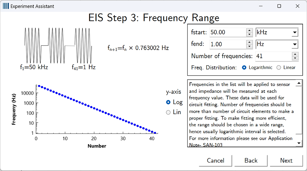
In logarithmic distribution, each frequency is a constant multiple of the previous frequency (in this case, 0.763×). This approach ensures equal representation across all frequency decades: if there are 10 frequencies between 1 Hz and 10 Hz, then 10 frequencies between 10 Hz and 100 Hz, and another 10 frequencies between 1 kHz and 10 kHz. This balanced distribution makes circuit analysis and fitting much more convenient and accurate. For this demonstration, we'll use the following frequency range settings:
Starting frequency: 50 kHz
Final frequency: 1 Hz
Distribution: 41 steps, logarithmically spaced
Notice that we start with high frequencies and progress to low frequencies. This approach offers several practical advantages. High-frequency measurements complete very quickly, allowing rapid assessment of experimental conditions. For example faulty cable connections become immediately apparent in high-frequency data, experimental setup errors manifest within seconds, problems can be identified and corrected before investing time in lengthy low-frequency measurements. If you started with low frequencies, it could take much longer to realize that something is wrong with your setup.

With our frequency range strategically distributed to capture all relevant electrochemical processes, we must now ensure our system reaches stable equilibrium before these measurements begin.
Step #4: Quiet time
Quiet time (also referred to as "wait time" or "equilibration time") is the pause period after applying your DC bias but before initiating the AC perturbation measurements. This waiting period allows the electrochemical system to reach a stable steady-state condition for making sure that your impedance data reflect equilibrium behavior rather than transient effects. When you apply a DC bias to your electrochemical system, several time-dependent processes occur, such as double layer charging and surface reactions. Without adequate quiet time, your impedance measurements will be contaminated by these transient effects, leading to inaccurate and irreproducible results. So, the goal is to ensure that your impedance data reflect the true steady-state electrochemical behavior of your system, free from charging currents, drift, or other time-dependent artifacts.
Since electrode charging follows exponential form, a commonly used guideline is to set the quiet time to 5 times the system's time constant. This ensures approximately 99.3% completion (1-(e^-5)) of the charging process. However, this theoretical approach has a practical limitation: we typically don't know the system's time constant beforehand, especially when characterizing new sensors or systems. The most reliable approach involves empirical testing through potentiometry by observing OCP vs time. For preliminary experiments or when time is limited, you can start with educated guesses. Quiet time optimization requires developing a strategy tailored to your specific application. For example, you can focus on high-frequency range since high-frequency impedance measurements are less affected by drift and transient effects, but you may miss important low-frequency information. Or alternatively you can wait until you're ensure complete system equilibration. But this increases total measurement time.
For this demonstration, we'll use a 1-second quiet time. This represents a reasonable starting point for many electrochemical systems, though optimization may be needed for your specific application.
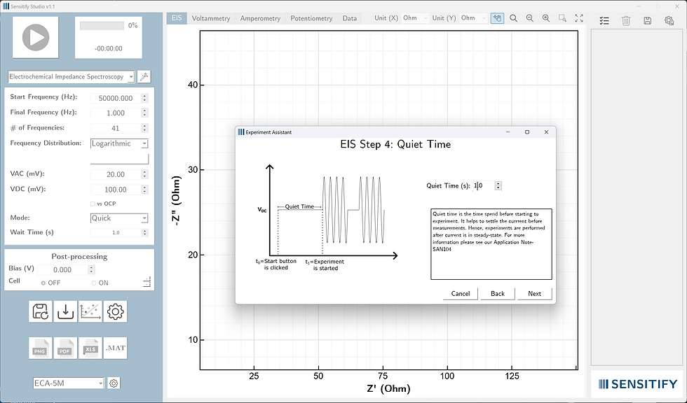
Click "Next" to proceed to post-processing.
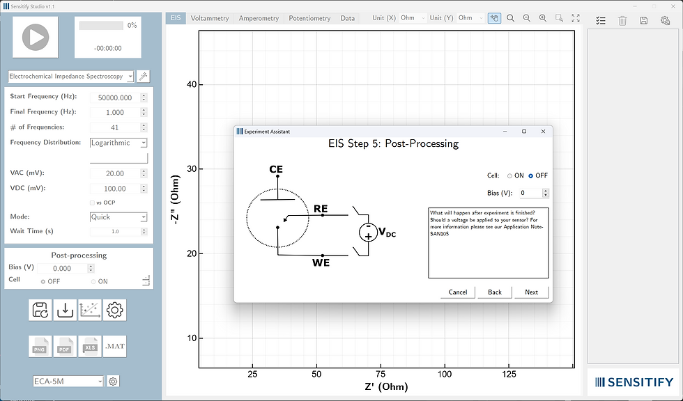
Step #5: Post-processing
After your EIS run completes, depending on the application, you can choose to apply some bias voltage. In post-processing section, you decide on this. For this demo we will choose "cell: off". Then click next.
Summary
In the summary page, you will see the summary of the chosen parameters. After you click "Finish", all the parameters will be set at the left panel.

Starting the experiment
After you click the start button, the experiment will start. See the below video showing all the steps.
References
Allan Bard, Larry Faulkner. Electrochemical methods: fundamentals and applications.
Mark Orazem, Bernard Tribollet. Electrochemical impedance spectroscopy.
